Exercise 1
Jai Broome
21 November, 2016
require(ggplot2)
require(dplyr)
require(knitr)
1 Simple Octave/MATLAB function
I’ll skip over this since I figure anyone wanting to follow along is already familiar with R
1.1 Submitting Solutions
You won’t be able to submit this for credit, but hopefully you still find this useful
2 Linear regression with one variable
Here I read in the data, split it into X and y, and generate starting values for theta
q1data <- read.table("data/ex1data1.txt",
                     sep = ",",
                     col.names = c("population", "profit"))
q1data$ones <- 1
q1data <- q1data %>% select(ones, population, profit)
X <- select(q1data, -profit)
y <- q1data$profit
theta <- rep(0, times = 2)
2.1 Plotting the Data
g1 <- ggplot(q1data, aes(x = population, y = profit)) +
    geom_point(shape = 4, color = "red", size = 3) +
    xlab("Population of City in 10,000s") +
    ylab("Profit in $10,000s")
g1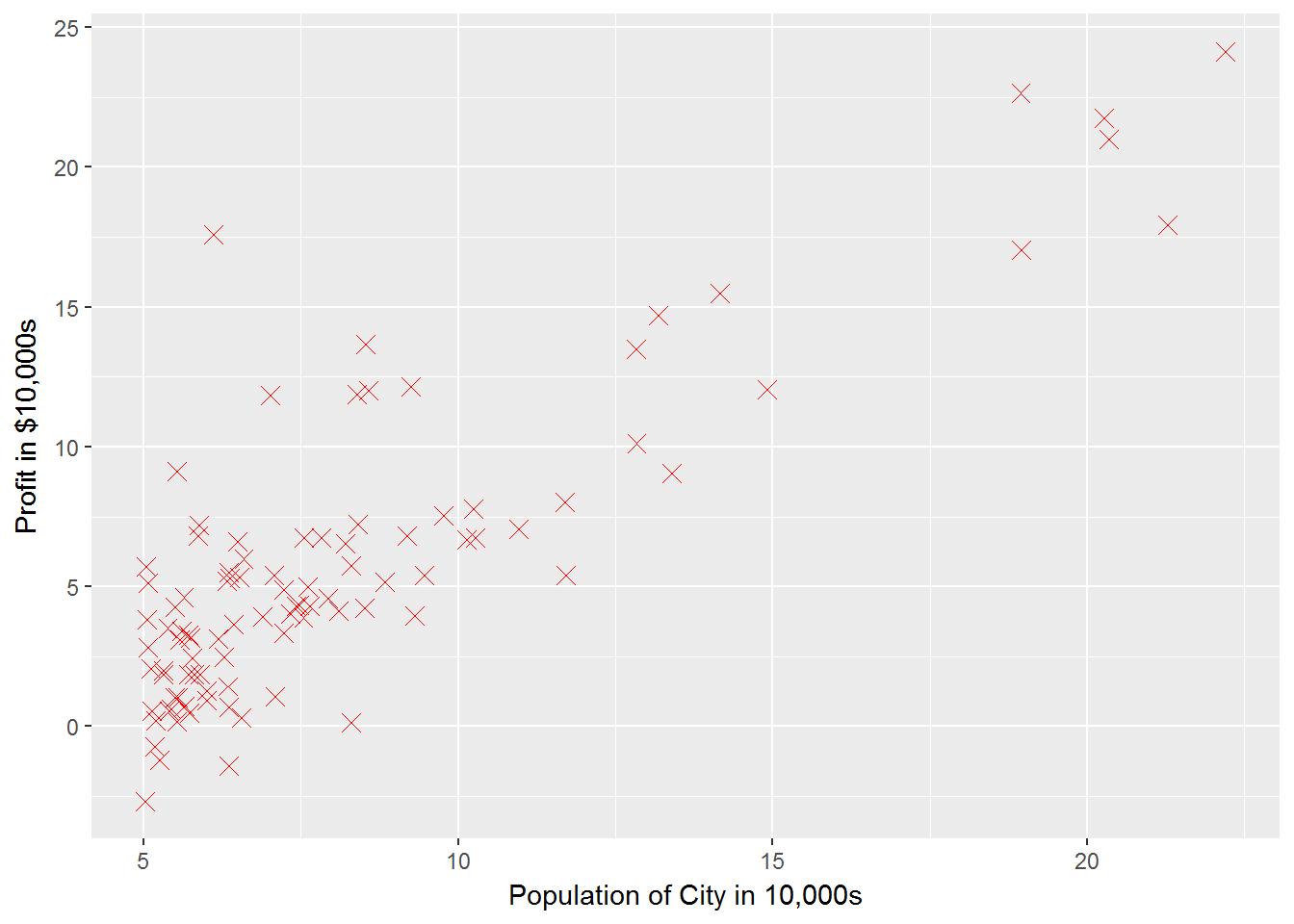
2.2 Gradient Descent
iterations <- 1500
alpha <- 0.01
Functions are defined in a separate script so they can be accessed for other assignments. See ?knitr::read_chunk
read_chunk("ex1/ex1_chunks.R")computeCost <- function(X, y, theta, lambda = 0){
if(is.null(dim(X))){
X <- t(data.frame(X))
}
m <- nrow(X)
pred <- theta %*% t(X)
sqError <- (pred - y) ^ 2
cost <- (1 / (2 * m)) * sum(sqError)
reg <- (lambda / (2 * m)) * sum(theta[-1]^2)
J <- cost + reg
gradient <- (1 / m) * sum((pred - y) * X[, 1]) # first element unregularized
for(j in 2:length(theta)){
gradient <- c(gradient, ((1 / m) * sum((pred - y) * X[, j]) + lambda * theta[j] / m))
}
return(list(J=J, gradient=gradient))
}gradStep <- function(thetaj, alpha, gradj){
thetaj - alpha * gradj
}Note that in the loop, thetas get stored in a temporary variable for simultaneous updating.
gradientDescent <- function(X, y, theta, alpha, iterations, lambda = 0){
    if(length(theta) != ncol(X)){stop("theta and X are nonconformable")}
    J_history <- data.frame()
    for (iteration in 1:iterations){

        a <- computeCost(X = X, y = y, theta = theta, lambda = lambda)
        J <- a$J
        gradient <- a$gradient
        J_history <- rbind(J_history, c(J, iteration - 1, theta))

        thetaTemp <- vector()
        for(j in 1:length(theta)){
            thetaTemp <- c(thetaTemp, gradStep(theta[j], alpha, gradient[j]))
        }
        theta <- thetaTemp
    }
    # for final iteration
    J <- computeCost(X = X, y = y, theta = theta, lambda = lambda)$J
    J_history <- rbind(J_history, c(J, iteration, theta))
    thetanames <- rep("theta", times = length(theta) - 1)
    for(i in length(thetanames)){thetanames[i] <- paste("theta", i, sep = "")}
    colnames(J_history) <- c("loss", "iterations", "theta0", thetanames)
    return(J_history)
}
computeCost(X, y, theta)## $J
## [1] 32.07273
##
## $gradient
## [1] -5.839135 -65.328850Should be 32.07
2.3 Debugging
Pay particular attention to indexing in these exercizes, because unlike Matlab, R does start indexing at 1
jhist <- gradientDescent(X, y, theta, alpha, iterations)
jhist <- jhist[2:(nrow(jhist) - 1),] #makes graph more interpretible
ggplot(jhist, aes(x = iterations, y = loss)) + geom_line()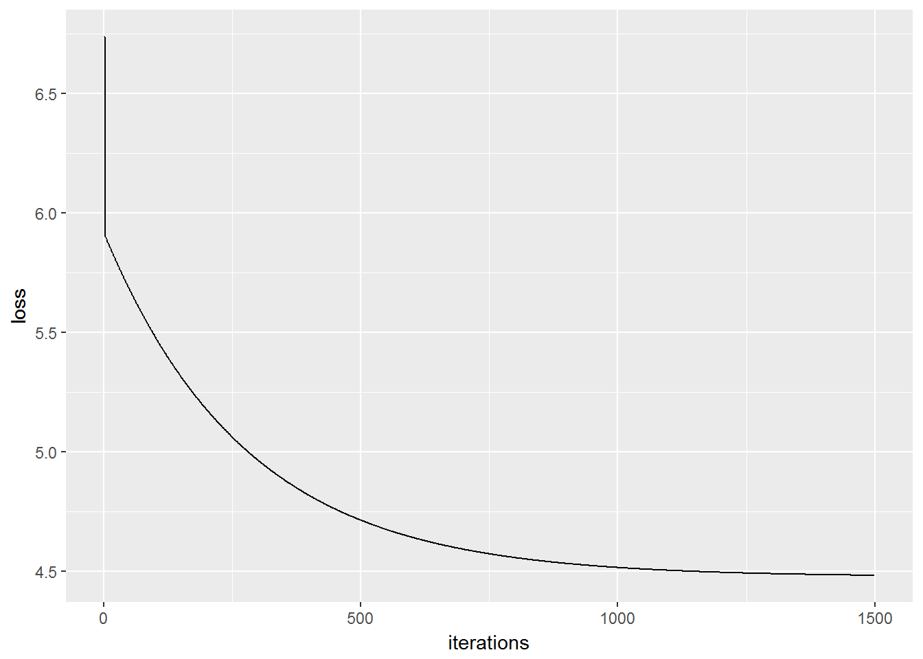
g1 + geom_abline(slope = tail(jhist$theta1, n = 1), intercept = tail(jhist$theta0, n = 1))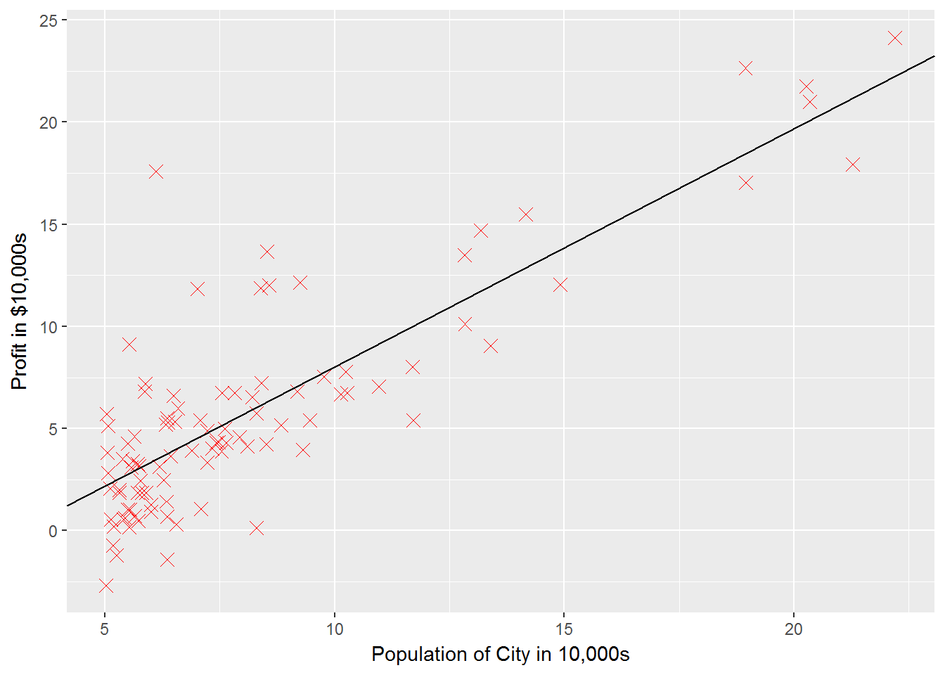
2.4 Visualizing \(J(\theta)\)
I skipped over this section since the code is already written in Matlab by the course instructors. See the assignment page for the images that show how different values of the thetas yield different costs
3 Optional exercises
These are still incomplete. I’m planning on returning to these after making it through the main course content